
前言
我们都知道,深度学习的成功的原因主要有两点:
- 当前计算机的计算能力有很大提升;
- 随着大数据时代的到来,当前的训练样本数目有很大的提升。
然而深度学习的一大问题是,有的问题并没有大量的训练数据,而由于深度神经网络具有非常强的学习能力,如果没有大量的训练数据,会造成过拟合,训练出的模型难以应用。因此对于一些没有足够样本数量的问题,可以通过已有的样本,对其进行变化,人工增加训练样本。
对于图像而言,常用的增加训练样本的方法主要有对图像进行旋转、移位等仿射变换,也可以使用镜像变换等等,这里介绍一种常用于字符样本上的变换方法,**弹性变换算法(Elastic Distortion)**。
该算法最先是由Patrice等人在2003年的ICDAR上发表的《Best Practices for Convolutional Neural Networks Applied to Visual Document Analysis》。本文主要是对论文中提出的弹性形变数据增强方法进行解读。
插播一下双线性插值的定义
- 双线性插值,顾名思义就是两个方向的线性插值加起来(这解释过于简单粗暴,哈哈)。所以只要了解什么是线性插值,分别在x轴和y轴都做一遍,就是双线性插值了。
- 线性插值:两个点A,B,要在AB中间插入一个点C(点C坐标在AB连线上),就直接让C的值落在AB的值的连线上就可以了。如A点坐标(0,0),值为3,B点坐标(0,2),值为5,那要对坐标为(0,1)的点C进行插值,就让C落在AB线上,值为4就可以了。
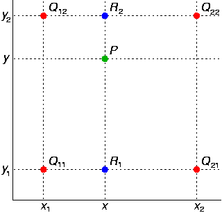
- 但是如果C不在AB的线上肿么办捏,所以就有了双线性插值。如下图,已知Q12,Q22,Q11,Q21,但是要插值的点为P点,这就要用双线性插值了,首先在x轴方向上,对R1和R2两个点进行插值,这个很简单,然后根据R1和R2对P点进行插值,这就是所谓的双线性插值。
1、仿射变换
- 仿射变换是最常用的空间坐标变换的方法之一,具体定义可参考冈萨雷斯的《数字图像处理第三版》50页。论文中是如下解释仿射变换的:
- 将仿射变换应用于图像,新像素的位置是由原始位置确定的,Δx(x,y)=1,Δy(x,y)=0代表向右移一个单位,Δx(x,y)= αx, Δy(x,y)= αy代表像素点由原点位置进行缩放。
- 上面说明了如何计算变换之后每个像素点的坐标,下图说明了如何应用位移字段来计算每个像素的新值(其实就是双线性插值的方法):
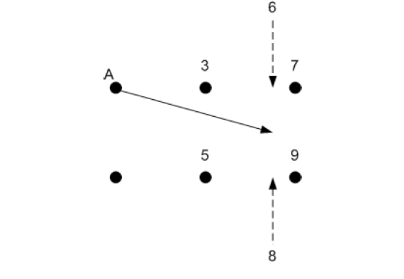
- 假设A是原点(0,0),而数字3,7,5,9是图像要转换的灰度等级,坐标分别为(1,0),(2,0),(1,-1),(1,-2),A的位移由Δx(0,0) = 1.75 and Δy(0,0) = -0.5给出,如箭头所示。通过评估原始图像的位置(1.75,-0.5)处的灰度级来计算新(扭曲)图像中的A的新灰度值。用于评估灰度级的简单算法是原始图像的像素值进行“线性插值”。尽管可以使用其他插值方案(例如,双三次和B样条插值),但双线性插值是最简单的插值方法之一,并且适用于以所选分辨率(29×29)生成附加的扭曲字符图像。
- 先水平插值,然后垂直插值,完成评估。箭头结束的位置在3,5,7,9的方格内,这样我们先计算箭头相对于它结束的方格的坐标。在这种情况下,它相对于正方形方格中的坐标是(0.75,0.5),假设该正方形的原点是左下角(也就是灰度值为5的点)。在此示例中,水平插值为:
3 +0.75×(7-3)= 6;垂直插值为:8 +0.5×(6-8)= 7,因此A的新像素值为7. - 对所有像素都进行了类似的计算。在给定图像之外的所有像素位置都假定有一个灰度值。
2、弹性形变
- 仿射变换改善了在MNIST数据集上的实验结果,但是实验在弹性形变后的数据集上取得了最好的结果。
那么什么是弹性形变呢?
- 首先创建随机位移场来使图像变形,即
Δx(x,y) = rand(-1,+1)、Δy(x,y)=rand(-1,+1),其中rand(-1,+1)是生成一个在(-1,1)之间均匀分布的随机数,然后用标准差为σ的高斯函数对Δx和Δy进行卷积,如果σ值很大,则结果值很小,因为随机值平均为0.如果我们将位移场标准化(达到1的范数),则该字段接近常数,具有随机方向。 - 如果σ很小,则归一化后该字段看起来像一个完全随机的字段(如图2右上角所示)。
- 对于中间σ值,位移场看起来像弹性变形,其中σ是弹性系数。然后将位移场乘以控制变形强度的比例因子α。 在我们的MNIST实验(29x29输入图像)中,产生最佳结果的值是σ = 4和α= 34。
- 将经过高斯卷积的位移场乘以控制变形强度的比例因子α,得到一个弹性形变的位移场,最后将这个位移场作用在仿射变换之后的图像上,得到最终弹性形变增强的数据。作用的过程相当于在仿射图像上插值的过程,最后返回插值之后的结果。
- 关于高斯卷积的原理可以参考这篇文章:高斯卷积滤波
- 如果文章看完文章,还是不太懂弹性形变数据增强的原理的话,可以结合代码一起看,下面是参考代码,我都有注释。
3、参考代码
# -*- coding:utf-8 -*-
"""
@author:TanQingBo
@file:elastic_transform.py
@time:2018/10/1221:56
"""
# Import stuff
import os
import numpy as np
import pandas as pd
import cv2
from scipy.ndimage.interpolation import map_coordinates
from scipy.ndimage.filters import gaussian_filter
import matplotlib.pyplot as plt

# Function to distort image  alpha = im_merge.shape[1]*2、sigma=im_merge.shape[1]*0.08、alpha_affine=sigma
def elastic_transform(image, alpha, sigma, alpha_affine, random_state=None):
    """Elastic deformation of images as described in [Simard2003]_ (with modifications).
    .. [Simard2003] Simard, Steinkraus and Platt, "Best Practices for
         Convolutional Neural Networks applied to Visual Document Analysis", in
         Proc. of the International Conference on Document Analysis and
         Recognition, 2003.
     Based on https://gist.github.com/erniejunior/601cdf56d2b424757de5
    """
    if random_state is None:
        random_state = np.random.RandomState(None)

    shape = image.shape
    shape_size = shape[:2]   #(512,512)表示图像的尺寸
    # Random affine
    center_square = np.float32(shape_size) // 2
    square_size = min(shape_size) // 3
    # pts1为变换前的坐标,pts2为变换后的坐标,范围为什么是center_square+-square_size?
    # 其中center_square是图像的中心,square_size=512//3=170
    pts1 = np.float32([center_square + square_size, [center_square[0] + square_size, center_square[1] - square_size],
                       center_square - square_size])
    pts2 = pts1 + random_state.uniform(-alpha_affine, alpha_affine, size=pts1.shape).astype(np.float32)
    # Mat getAffineTransform(InputArray src, InputArray dst)  src表示输入的三个点,dst表示输出的三个点,获取变换矩阵M
    M = cv2.getAffineTransform(pts1, pts2)  #获取变换矩阵
    #默认使用 双线性插值,
    image = cv2.warpAffine(image, M, shape_size[::-1], borderMode=cv2.BORDER_REFLECT_101)

    # # random_state.rand(*shape) 会产生一个和 shape 一样打的服从[0,1]均匀分布的矩阵
    # * 2 - 1 是为了将分布平移到 [-1, 1] 的区间
    # 对random_state.rand(*shape)做高斯卷积,没有对图像做高斯卷积,为什么?因为论文上这样操作的
    # 高斯卷积原理可参考:https://blog.csdn.net/sunmc1204953974/article/details/50634652
    # 实际上 dx 和 dy 就是在计算论文中弹性变换的那三步:产生一个随机的位移,将卷积核作用在上面,用 alpha 决定尺度的大小
    dx = gaussian_filter((random_state.rand(*shape) * 2 - 1), sigma) * alpha
    dy = gaussian_filter((random_state.rand(*shape) * 2 - 1), sigma) * alpha
    dz = np.zeros_like(dx)  #构造一个尺寸与dx相同的O矩阵
    # np.meshgrid 生成网格点坐标矩阵,并在生成的网格点坐标矩阵上加上刚刚的到的dx dy
    x, y, z = np.meshgrid(np.arange(shape[1]), np.arange(shape[0]), np.arange(shape[2]))  #网格采样点函数
    indices = np.reshape(y + dy, (-1, 1)), np.reshape(x + dx, (-1, 1)), np.reshape(z, (-1, 1))
    # indices = np.reshape(y+dy, (-1, 1)), np.reshape(x+dx, (-1, 1)), np.reshape(z, (-1, 1))
    return map_coordinates(image, indices, order=1, mode='reflect').reshape(shape)

# Define function to draw a grid
def draw_grid(im, grid_size):
    # Draw grid lines
    for i in range(0, im.shape[1], grid_size):
        cv2.line(im, (i, 0), (i, im.shape[0]), color=(255,))
    for j in range(0, im.shape[0], grid_size):
        cv2.line(im, (0, j), (im.shape[1], j), color=(255,))

if __name__ == '__main__':
    img_path = 'E:/liverdata/nii/png/img'
    mask_path = 'E:/liverdata/nii/png/label'
    # img_path =  '/home/changzhang/ liubo_workspace/tmp_for_test/img'
    # mask_path = '/home/changzhang/liubo_workspace/tmp_for_test/mask'
    img_list = sorted(os.listdir(img_path))
    mask_list = sorted(os.listdir(mask_path))
    print(img_list)
    img_num = len(img_list)
    mask_num = len(mask_list)
    assert img_num == mask_num, 'img nuimber is not equal to mask num.'
    count_total = 0
    for i in range(img_num):
        print(os.path.join(img_path, img_list[i]))   #将路径和文件名合成一个整体
        im = cv2.imread(os.path.join(img_path, img_list[i]), -1)
        im_mask = cv2.imread(os.path.join(mask_path, mask_list[i]), -1)
        # # Draw grid lines
        # draw_grid(im, 50)
        # draw_grid(im_mask, 50)
        # Merge images into separete channels (shape will be (cols, rols, 2))
        im_merge = np.concatenate((im[..., None], im_mask[..., None]), axis=2)
        # get img and mask shortname
        (img_shotname, img_extension) = os.path.splitext(img_list[i])  #将文件名和扩展名分开
        (mask_shotname, mask_extension) = os.path.splitext(mask_list[i])
        # Elastic deformation 10 times
        count = 0
        while count < 10:
            # Apply transformation on image  im_merge.shape[1]表示图像中像素点的个数
            im_merge_t = elastic_transform(im_merge, im_merge.shape[1] * 2, im_merge.shape[1] * 0.08,
                                           im_merge.shape[1] * 0.08)

            # Split image and mask
            im_t = im_merge_t[..., 0]
            im_mask_t = im_merge_t[..., 1]
            # save the new imgs and masks
            cv2.imwrite(os.path.join(img_path, img_shotname + '-' + str(count) + img_extension), im_t)
            cv2.imwrite(os.path.join(mask_path, mask_shotname + '-' + str(count) + mask_extension), im_mask_t)
            count += 1
            count_total += 1
        if count_total % 100 == 0:
            print('Elastic deformation generated {} imgs', format(count_total))
            # # Display result
            # print 'Display result'
            # plt.figure(figsize = (16,14))
            # plt.imshow(np.c_[np.r_[im, im_mask], np.r_[im_t, im_mask_t]], cmap='gray')
            # plt.show()
- 关于map_coordinates函数原理的参考文章:Python/Scipy插值(map_coordinates)